Unleash Pandas: All You Need to Master Data

Why do we need Pandas?

Well, Excel is good for getting things done. However, I believe Excel has its limitations, beyond which it no longer makes sense to use. For instance, I regularly receive monthly data updates from clients in Excel, which I need to compare with the existing version to identify changes. It’s manageable with 1 or 2 columns, but with more, repeating the task becomes inefficient. This is where Pandas step in!!

I have automated the task using Python and Pandas, and now by the time I look up a column in Excel, I have the report ready with Python.

Pandas is a Python package, which makes working with tables easier, and It has much more flexibility and control than Excel, making it a favourite choice for Data scientists.

Why learning about Pandas is important for data scientists?
Pandas is a fast and powerful data analysis tool. It is also widely popular that many machine learning frameworks are built, to support it. So, learning about pandas and the variety of functionality it offers, makes our jobs easier.

Let’s dive in and explore the basics to get started.

How to install

Installing pandas is very easy if you are using Python with Anaconda/Miniconda or PyPI. If you don’t have these already, I highly recommend using Anaconda as it is helpful, for managing code environments. 

I would recommend Anaconda to new users as it is easy to use. Miniconda is a light version of an Anaconda, without UI and terminal-based. So, I suggested it for advanced users only.

For Installing Anaconda:

Install with Anaconda/Miniconda:

1. Open the Anaconda prompt, if you are using Windows/MacOS. If you are using Linux/Miniconda open the terminal and run conda init.
2. Run the following command in the terminal

conda install -c conda-forge pandas -y

If you prefer PyPI:

1. Open your terminal, and make sure pip is installed along with Python.
2. Run the following command

pip install pandas

Additional tip: 
To install specific versions of pandas you can use
pandas==<version_number>.

Test Installation

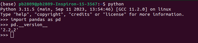
To test the installation, import pandas and check it version to see the installed version.

Getting Started

Data Structure

Pandas has two types of data structures: Series and DataFrame 

Series: 1D array, which can store homogeneously typed(all data is of same data type) data.

DataFrame: 2D data, generally a collection of series. We can assign different series with different data types in a data frame.

Pandas allows two data structures to allow more flexibility in storing different data types in one table.

Properties

1. DataFrames/Series are value-mutable(data can be changed after creation).
2. They are not always size-mutable. we cannot alter the length of the series in DataFrame, but we cannot add a new column.
3. Most in-built methods allow control, to edit the current object or create a copy.
4. The data can be accessed using dictionary-like syntax.
   Ex: sample_df[‘series_1’]: We can use this code for accessing Series with name series_1 in DataFrame named sample_df.

Basic Syntax:

To understand how pandas works, and understand its syntax, let us take a sample file and work through it.

Download the file from here

The file contains 10 rows and 8 columns of data and they are described below:

1. ID: Unique identifier for each employee.
2. Name: Name of the employee.
3. Age: Age of the employee.
4. Salary: Annual salary of the employee (in USD).
5. Join_Date: The date when the employee joined the company.
6. Is_Manager: Boolean value indicating if the employee holds a managerial position.
7. Department: The department the employee belongs to (e.g., HR, Finance, IT, Marketing).
8. Rating: Performance rating of the employee (on a scale of 1-5)

First thing first, let us import pandas and read the file.

import pandas as pd	
df = pd.read_csv('sample_dataset_pandas.csv')

This command will read the CSV file named sample_dataset_pandas.csv and load it into df. Function read_csv by default assumes the first column in the data as column headers. Let’s check the shape and column available in df to make sure the data is read correctly:

size = df.shape # used to get shape of dataframe
print(f'Num of rows: {size[0]}')
print(f'Num of columns: {size[1]}')


columns_available = df.columns.to_list() 
# columns-method to get column headers in dataframe, to_list - get them as list
print(f'Columns available in data: {", ".join(columns_available)}')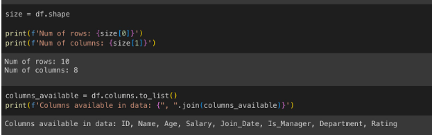

We can confirm that the data is loaded correctly and all columns are available. Now, we can quickly check the data types of all columns.

df.info()

We can see that the table contains multiple data types. But did you observe that Join_Date is an object data type? Pandas have built-in capabilities to support datetime formats. Let’s quickly convert them to dates.

df['Join_Date'] = pd.to_datetime(df['Join_Date'])
print(f"Now column is of datatype: {df['Join_Date'].dtypes}, Example: {df['Join_Date'].iloc[0]}")
print()
df['Join_Date'] = pd.to_datetime(df['Join_Date']).dt.date
print(f"Example: {df['Join_Date'].iloc[0]}")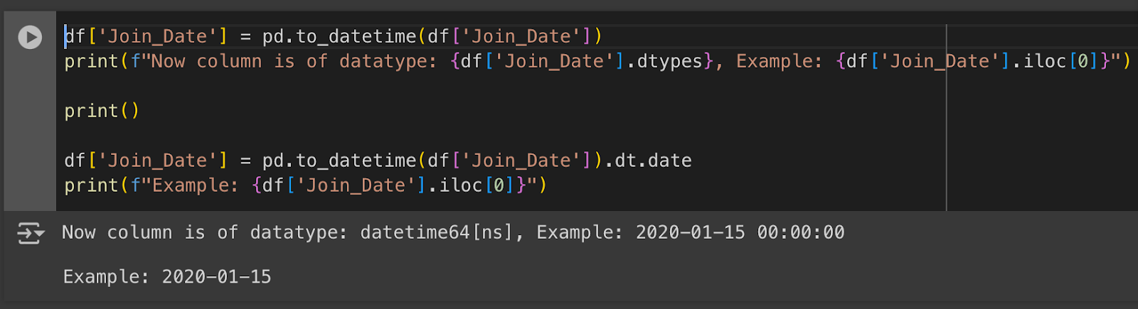

When converted using pd.to_datetime, the underlying data type is datetime64[ns], which stores date and time as shown above. If you need only dates, you can use the dt package from Pandas. Note, after using the dt package data type will be object, but the underlying properties are of datetime.

Now, if I need to calculate no of days since joining for all employees, it’s easy as I can perform column-level operations.

df['No. of days since joining'] = (pd.to_datetime('today').date() - df['Join_Date']).apply(lambda x: x.days)
# .apply is not needed if you use datetime64[ns] datatype, you can use .dt.days
df['No. of days since joining'].describe()

Did you observe how easily we got the statistics of a numerical column using the described method?

Pandas also allows the creation of new columns effortlessly, we created a new column in the dataframe and put in new data. You can create a new column with a custom input of your own.

print(f'NUmber of columns before adding: {df.shape[1]}')
df['New column']=['some','random','data',None,None,'some','more','random','data',None]
# df['New column'] = 4 #if you want to give a constant input
# df['New column'] = list # data stored in another array as input
# Please note: if adding a new column using array data, shape of array should be same # as number of rows on table
print(f'NUmber of columns after adding: {df.shape[1]}')
df.drop('New column', axis=1, inplace=True)
# axis=1 indicates columns, inplace=true means drop in current object only and don't 
# create a copy
print(f'NUmber of columns after dropping: {df.shape[1]}')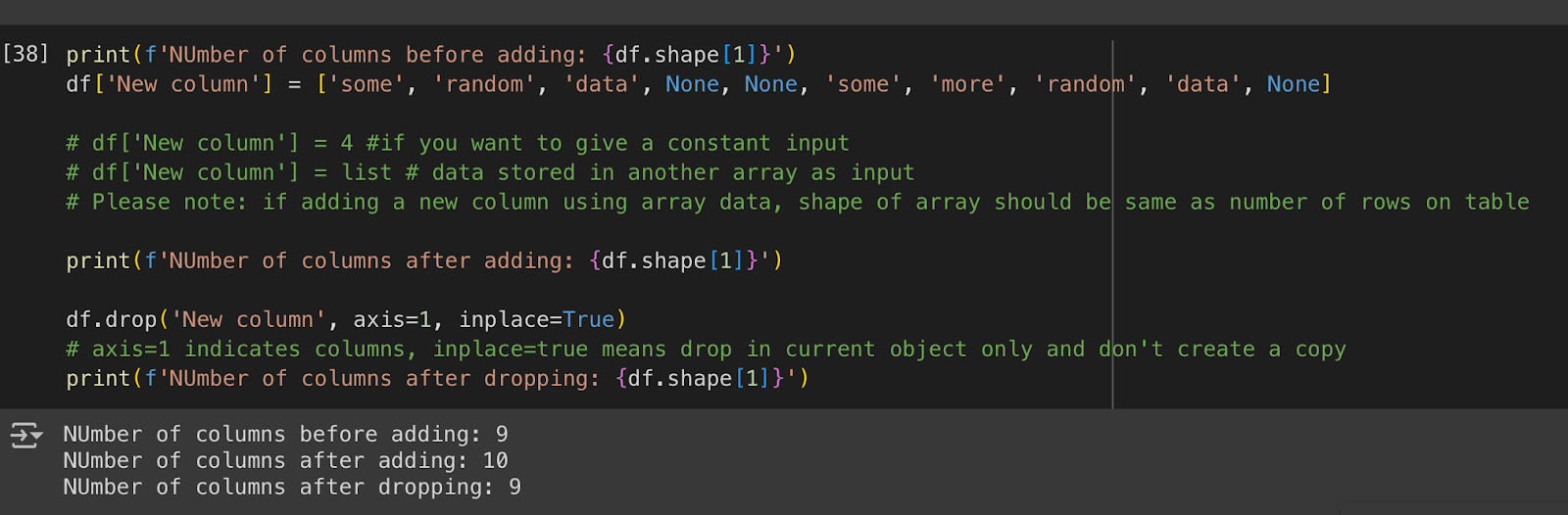

Adding and dropping a column was so easy!

Read API Documentation

Pandas library is vast and I have just covered a glimpse. But, I will let you know how to read its API documentation to understand the available methods, their parameters, attributes and what it returns.

I will explain a sample API documentation here and leave the rest to you. We will look at a function called fillna(), which can fill null/missing values in a table. Documentation for this can be accessed here.
The function has a call sign as pandas.DataFrame.fillna, indicates that this method applies to the DataFrame object in Pandas, and we cannot use it in series or other objects.

Then we can find a brief description of what the function does:

• Fill NA/NaN values using the specified method

Then we can find the parameters available: value, method, axis, inplace, limit, and downcast. Let’s look at the value parameter explanation.

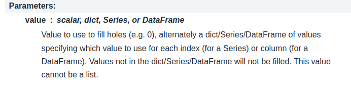
Parameter: Value

Accepted Data types: scalar, dict, Series, or DataFrame

Description: Value to use to fill holes (e.g. 0), alternately a dict/Series/DataFrame of values specifying which value to use for each index (for a Series) or column (for a DataFrame). The function does not fill values that are not in the dict/Series/DataFrame. This value cannot be a list.

Next, the return section specifies what we receive after the function executes. If you scroll further below, we can also find an example section on the usage of the function. 

Although we cannot cover all the methods available using this approach, you can understand any function available in pandas using their official API reference documentation found here.