
Picture yourself as a fortune teller, peering into a crystal ball to see what the future holds. But instead of some mystical ability, you’ve got a treasure trove of data at your fingertips! Welcome to the intriguing realm of time series modeling, where we turn past data into insightful forecasts that empower businesses to make smart choices. Whether you’re looking to predict stock trends, sales numbers, or even the weather, time series analysis is your reliable companion.
In this blog, we’re going to explore a variety of time series modeling techniques, like Moving Average (MA), Exponential Smoothing, ARIMA, SARIMA, Prophet, and LSTM. Each method has its special touch and is perfect for different kinds of data and forecasting challenges. So, put on your data glasses, and let’s jump into the wonders of time series modeling!
Understanding Time Series Modeling
Time series modeling is a cool statistical method that helps us look at and forecast from the data collected over time. If you’re just getting started with this idea, no need to stress! Let’s simplify it.
Time series modeling is all about collecting data points at consistent intervals—think daily stock prices, monthly sales, or yearly rainfall—and using that info to forecast what might happen next. The important thing to remember about time series data is that it’s arranged in chronological order, so the sequence in which the data is collected counts. In statistical terms, the proper definition of the time series model is –
A time series model consists of a sequence of data points arranged chronologically, with time serving as the independent variable. Such models are employed for analysis and prediction of future trends.
Before jumping into the core of time series modeling, let us understand the additional factors to consider when analyzing time series data. Is the series stationary? Does it exhibit seasonality? Is there autocorrelation present in the target variable?
Stationarity
It refers to the condition in which the statistical characteristics of a dataset remain unchanged over time. This encompasses several key aspects:
1. Mean: The average value of the dataset is stable.
2. Variance: The degree of variability or dispersion within the dataset remains consistent.
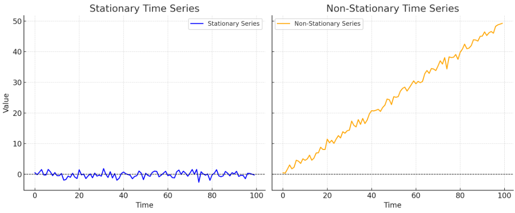
Many time series modelings, such as ARIMA, perform better when the data is stationary. When the data isn’t stationary, it can result in inaccurate forecasts. Imagine this: if you were trying to guess tomorrow’s temperature using past temperatures, but the average temperature keeps increasing each year (for instance, due to climate change), your predictions would be incorrect since the average is shifting. Here is a graph demonstrating the difference between stationary and non-stationary time series:
Non-Stationary Time Series: Includes a trend, showing changes in mean over time
Stationary Time Series: Random noise with constant mean and variance.
Techniques To Achieve Stationarity
To make a time series stationary from non-stationary we can use various techniques. Let’s look into a few of them and try to understand how they work-
1. Differencing – It allows us to eliminate trends in data. Differencing means taking the current observation and subtracting the one before it. For instance, if yt is the value at time t, the first difference is computed as:

2. Log Transformation – Transforming the data using logarithms can help even out the variance. This is especially handy for data that grows exponentially. For example, if you have the original series as yt , the new series after transformation would be:

3. Seasonal Differencing – If the data exhibits seasonality, subtracting the value from the same season in the previous cycle can help. For example:

Code
Let’s look into some code and see the execution of differencing-
import pandas as pd
import numpy as np
import matplotlib.pyplot as plt

# Create a sample time series data for 2 years
data = {
    'Month': pd.date_range(start='2020-01-01', periods=24, freq='M'),
    'Sales': [100, 110, 120, 130, 140, 150, 160, 175, 180, 190, 200, 210,
              220, 230, 240, 250, 260, 270, 280, 295, 300, 310, 320, 330]
}

# Create a DataFrame
df = pd.DataFrame(data)
df.set_index('Month', inplace=True)

# Display the original series
print("Original Series:")
print(df)

# First Differencing
df['First_Difference'] = df['Sales'].diff()

# Seasonal Differencing (assuming monthly data with a seasonality of 12 months)
df['Seasonal_Difference'] = df['Sales'].diff(12)

# Display the results
print("\nDifferenced Series:")
print(df)

# Plotting the original and differenced series
plt.figure(figsize=(14, 10))

plt.subplot(3, 1, 1)
plt.plot(df['Sales'], marker='o', label='Original Sales')
plt.title('Original Sales Data')
plt.legend()

plt.subplot(3, 1, 2)
plt.plot(df['First_Difference'], marker='o', color='orange', label='First Difference')
plt.title('First Differenced Sales Data')
plt.legend()

plt.subplot(3, 1, 3)
plt.plot(df['Seasonal_Difference'], marker='o', color='green', label='Seasonal Difference')
plt.title('Seasonal Differenced Sales Data')
plt.legend()

plt.tight_layout()
plt.show()
The code contains some essential libraries: pandas for handling data, NumPy for any numerical tasks, and matplotlib.pyplot for creating plots. Then a dataset that includes monthly sales figures spanning two years has been generated.
The first difference is calculated using the diff() method where a seasonal differencing is performed by specifying a lag of 12 (for monthly data).

Seasonality
It refers to the idea that specific events or trends happen repeatedly over certain time frames, like daily, weekly, monthly, or yearly. Different elements, such as weather changes, holidays, or economic cycles, can influence these recurring patterns. Identifying these trends is crucial for making precise predictions and smart choices in different areas, like retail and energy management. By grasping the concept of seasonality and tweaking your models to fit, you can enhance your ability to forecast future developments.
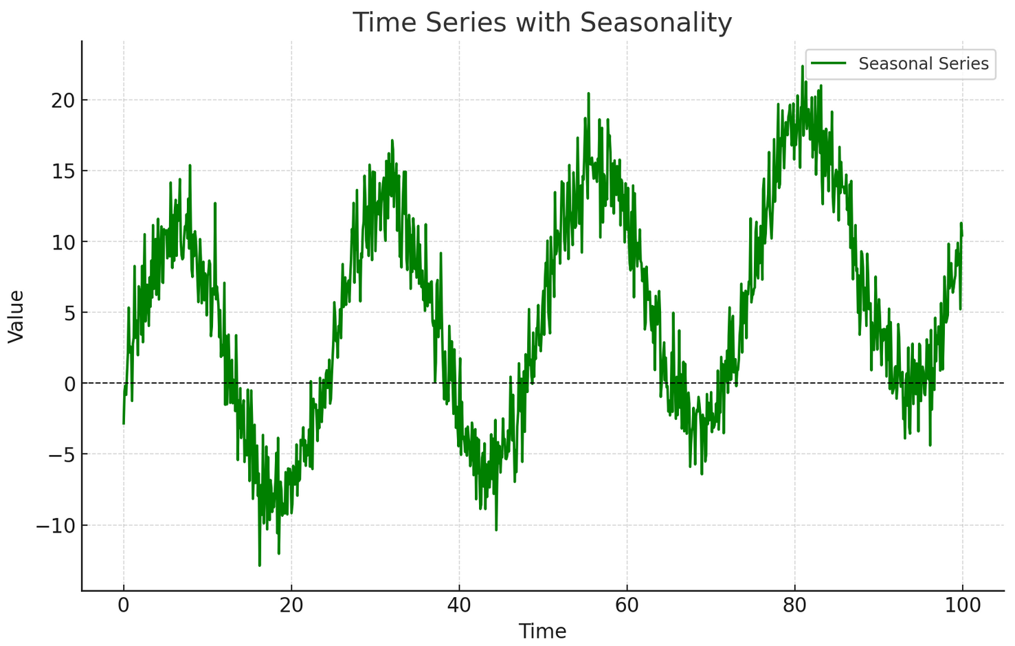
Here is a graph illustrating seasonality in a time series:
Seasonal Pattern: A repeating sinusoidal pattern over fixed intervals.
Trend: A slight upward trend was added to mimic real-world scenarios.
Autocorrelation
It refers to the correlation of a time series with its past values. It helps us identify patterns and dependencies within the data. For example, if today’s temperature is similar to yesterday’s temperature, we can say there is a positive autocorrelation at a lag of one day. Now here are two terms that might interest you: Lag and correlation.
Lag: This term describes how many periods you go back to find a connection. For example, a lag of 1 in daily timeframe indicates you’re looking at today’s value compared to yesterday’s, while a lag of 2 means you’re comparing today’s value with the value from two days ago.
Correlation Coefficient: This is a number that ranges from -1 to 1 and shows how strong and in what direction two values are related. A positive number means that when one value goes up, the other usually goes up too, while a negative number means they move in opposite directions.
Here is an autocorrelation plot, which shows the correlation of a time series with its own lagged values:
X-axis: Lag values.
Y-axis: Autocorrelation coefficients, which indicate the strength of correlation at each lag.

Time Series Modeling Techniques
The Moving Average
This model is a basic technique used in time series analysis. It forecasts future values by averaging past data points within a certain timeframe. This approach helps to reduce short-term variations and emphasizes long-term patterns.
For instance, think about a retail shop looking at its weekly sales figures. By using a moving average of the past four weeks, the shop can estimate next week’s sales by looking at the recent trends.
import pandas as pd

# Sample data
data = {'Week': [1, 2, 3, 4, 5, 6],
        'Sales': [200, 220, 250, 270, 300, 320]}
df = pd.DataFrame(data)

# Calculate moving average
df['Moving_Average'] = df['Sales'].rolling(window=4).mean()
print(df)
OUTPUT – The output shows the original sales data and the calculated moving averages, with NaN for the first three weeks (not enough data).

Exponential Smoothing
It applies weights to historical data that decrease exponentially over time. This approach ensures that more recent data points have a stronger impact on the forecast compared to older data. There are three primary forms of exponential smoothing:
1. Simple Exponential Smoothing: Ideal for datasets that do not exhibit trends or seasonal variations.
2. Holt’s Linear Trend Model: Appropriate for datasets that display trends.
3. Holt-Winters Seasonal Model: Designed for datasets that show both trends and seasonal patterns.
For instance, a financial analyst may utilize the Holt-Winters model to predict monthly revenue that follows seasonal fluctuations.
from statsmodels.tsa.holtwinters import ExponentialSmoothing

# Sample data
sales_data = [200, 220, 250, 270, 300, 320]
model = ExponentialSmoothing(sales_data, seasonal='add', seasonal_periods=2) # Changed seasonal_periods to 2
fit = model.fit()
forecast = fit.forecast(steps=2)
print(forecast)
OUTPUT- The output from the Exponential Smoothing model provides forecasted values for the next two time periods based on historical sales data.

ARIMA – AutoRegressive Integrated Moving Average
ARIMA, which stands for AutoRegressive Integrated Moving Average, is a widely utilized statistical technique for forecasting time series data. It integrates three key elements:
1. AR (AutoRegressive): This component relies on the dependent variable historical values.
2. I (Integrated): This involves differencing the data to achieve stationarity.
3. MA (Moving Average): This aspect considers previous forecast errors.
ARIMA is particularly effective for non-seasonal univariate time series datasets. For instance, a business could apply ARIMA to predict quarterly sales by analyzing historical sales figures.
from statsmodels.tsa.arima.model import ARIMA

# Sample data
sales_data = [299, 220, 250, 270, 300]
model = ARIMA(sales_data, order=(1,1,1))
fit = model.fit()
forecast = fit.forecast(steps=2)
print(forecast)
OUTPUT- The output indicates that the model predicts sales will be approximately 274 units in the next period and 270 units in the following period.

SARIMA (Seasonal ARIMA)
SARIMA enhances the ARIMA model by incorporating seasonal elements. It introduces extra parameters to capture the seasonal variations present in the data. Real-life Example: A tourism board might utilize SARIMA to forecast monthly visitor counts that exhibit seasonal trends influenced by holidays and events.
from statsmodels.tsa.statespace.sarimax import SARIMAX

# Sample seasonal data
seasonal_data = [100 + i*10 for i in range(12)] # Simulated monthly data
model = SARIMAX(seasonal_data, order=(1,1,1), seasonal_order=(1,1,1,12))
fit = model.fit()
forecast = fit.forecast(steps=3)
print(forecast)
OUTPUT- The output shows the predicted values for the next three periods (in this case, months)

Prophet
Prophet, created by Facebook, is tailored for predicting time series data characterized by significant seasonal variations and extensive historical records. It is designed to be intuitive and effectively handles missing values and anomalies. For instance, an online retail platform might utilize Prophet to project sales during holiday periods, where the patterns are intricate and fluctuate considerably. Let’s look into some code!
!pip install prophet
#from fbprophet import Prophet # Original line causing the error
from prophet import Prophet # Updated import statement
# Prepare your dataframe with 'ds' and 'y'
import pandas as pd
import numpy as np # Make sure to import numpy
df = pd.DataFrame({'ds': pd.date_range(start='2020-01-01', periods=100),
'y': np.random.rand(100)})
model = Prophet()
model.fit(df)
future = model.make_future_dataframe(periods=30)
forecast = model.predict(future)
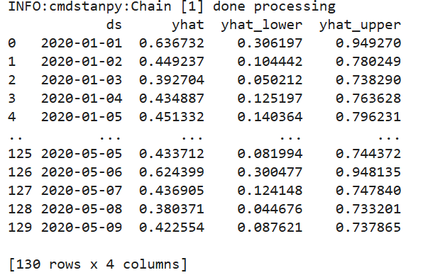
print(forecast[['ds', 'yhat', 'yhat_lower', 'yhat_upper']])OUTPUT – The output from the Prophet model will display a dataframe with the following columns for each date in the forecast period:
ds: The date of the forecast.
yhat: The predicted value for that date.
yhat_lower: The lower bound of the uncertainty interval for the prediction.
yhat_upper: The upper bound of the uncertainty interval for the prediction.
Predicted Values: The yhat column displays the model’s projections for upcoming values.
Uncertainty Intervals: The yhat_lower and yhat_upper columns offer a range that reflects the uncertainty associated with each forecast, aiding in the comprehension of possible variations in future results.
LSTM – Long Short-Term Memory
It is a specialized form of recurrent neural network (RNN) that excels in addressing sequence prediction challenges, including time series forecasting. These models are capable of capturing long-term dependencies within sequential datasets. A practical application can be a technology firm that may implement LSTM models to forecast server load by analyzing historical usage trends.
import numpy as np
from keras.models import Sequential
from keras.layers import LSTM, Dense

# Prepare your dataset
data = np.array([i for i in range(100)])
# Adjusted reshaping to create overlapping sequences
X_train = []
y_train = []
for i in range(10, len(data)):
    X_train.append(data[i-10:i])
    y_train.append(data[i])
X_train, y_train = np.array(X_train), np.array(y_train)
X_train = X_train.reshape(X_train.shape[0], X_train.shape[1], 1)  # Reshape for LSTM input


# Build LSTM model
model = Sequential()
model.add(LSTM(50, activation='relu', input_shape=(X_train.shape[1], X_train.shape[2])))
model.add(Dense(1))
model.compile(optimizer='adam', loss='mse')

# Fit model
model.fit(X_train, y_train, epochs=200)
OUTPUT- The provided code snippet builds and trains an LSTM (Long Short-Term Memory) neural network model using Keras to predict the next value in a sequence based on the previous 10 values.


What does the output indicate?
Loss Value: The decreasing loss value indicates that the model is learning and improving its predictions over the epochs.
Epochs: The number of epochs shows how many times the model has gone through the entire training dataset.
Check out more on – Predictive Analysis.
Conclusion
Time series modeling is an essential tool for analyzing and forecasting data over time. In this blog, we explored various methods such as Moving Average, Exponential Smoothing, ARIMA, SARIMA, Prophet, and LSTM, each suited for different forecasting needs.
Key concepts like stationarity, seasonality, and autocorrelation are vital for effective analysis. By understanding these patterns in historical data, you can make informed predictions about future trends. Whether you’re in business, finance, or research, mastering time series modeling enhances your decision-making capabilities. In a data-driven world, leveraging these insights can help you stay ahead and drive success.